Table of Contents
The article below is based off of chapter 2 of the FastAI textbook. I’ll be writing about whatever I learned from it.
I’m new to all of this! If anything here is incorrect or could be improved, please let me know!
1.0: Purpose
Using the FastAI library, we’re going to write a classifier that classifies bears! After that, we’ll see what we can do with our newfound knowledge.
I’ll be doing the following in Google Colab.
2.0: Setup
First, we’ll import the libraries we’ll need:
1! [ -e /content ] && pip install -Uqq fastbook
2import fastbook
3fastbook.setup_book()
4from fastbook import *
5from fastai.vision.widgets import *
6!pip install -Uqq ddgs
7from ddgs import DDGS
If you’re doing this in Google Colab, then you’ll probably be prompted to allow it to access your Google Drive.
3.0: Acquiring our data
In order to train our AI model, we’ll need images of bears. For this purpose, we’ll work on classifying 3 categories of bears:
- grizzly bears
- black bears
- teddy bears
In order to acquire these images, we’ll need to scrape them off of the internet. The textbook uses the Microsoft Bing API, but since I don’t like Microsoft, we’ll use duckduckgo instead (which is why we imported the ddgs package above). I’m not proficient with the ddgs library, so I adapted some code from this Kaggle notebook and used a fix from what is currently the top comment on this video. Our image scraping code looks as such:
1def search_images(keywords, max_images = 30): # max_images will default to 30
2    return L(DDGS().images(keywords, max_results=max_images)).itemgot('image')
Now we’ll use this code to download 100 images to a /bears directory.
1bear_types = ('grizzly', 'black', 'teddy')
2image_download_path = Path('bears')
3
4if not image_download_path.exists():
5    image_download_path.mkdir()
6    for bear_type in bear_types:
7        download_destination = (image_download_path/bear_type)
8        download_destination.mkdir(exist_ok=True)
9        download_images(download_destination, urls=search_images(f"{bear_type} bear", max_images=100))
Let’s check if any images are corrupt and remove them:
1image_files = get_image_files(image_download_path)
2corrupt_images = verify_images(image_files)
3corrupt_images.map(Path.unlink)
4.0: What on earth is DataLoaders?
This is a class that provides your AI model with the data required to train it. What we’re going to do here is create a DataBlock which we’ll then use to create a DataLoaders object. This DataBlock object is going to provide the images we downloaded to the DataLoaders object which will then pass it to the AI model for training purposes. Here’s what this looks like in code:
1bears = DataBlock(
2    blocks = (ImageBlock, CategoryBlock),
3    get_items = get_image_files,
4    splitter = RandomSplitter(valid_pct = 0.2, seed = 42),
5    get_y = parent_label,
6    item_tfms = Resize(128)
7)
Let’s run through the parameters we’ve passed above:
blocks = (ImageBlock, CategoryBlock)- This piece defines the input and output data. We’re passing images into the model and we want categories out of the model (predict the type of bear based on an image, right?).
get_items = get_image_files- This piece will obtain all of the images we downloaded and store it in the
DataBlock.
- This piece will obtain all of the images we downloaded and store it in the
splitter = RandomSplitter(valid_pct = 0.2, seed = 42)- This will split our data into two partitions: a training set and validation set.
- The training set is used to, well, train the model.
- The validation set is used to test the accuracy of our model.
valid_pct = 0.2tells ourDataBlockto set aside 20% of our input data for validation purposes.seed = 42ensures the same splitting occurs each time theDatablockis created. The seed doesn’t have to be 42.
- This will split our data into two partitions: a training set and validation set.
get_y = parent_label- This will get the possible predictions our model can make. In this case, since our images are stored in folders that correspond to the type of bear, the possible predictions are the types of bears.
- This parameter is called
get_ybecause we can think of our AI model as a graph with a cartesian plane. The $x$ axis denotes the independent variable, in this case, the images we’re providing to the model. Thus, the $y$ axis denotes the dependent variable, or the predictions of the model (based on the input data).
item_tfms = Resize(128)item_tfmsis short for item transformations. The transformation we’re applying here is resizing the image to 128x128 px. By default, theResize()function will crop the images to fit that size.
Now, we’ll create a DataLoaders object from our DataBlock and point it to the images we downloaded.
1bear_dataloaders = bears.dataloaders(image_download_path)5.0: Data augmentation
What we’re going to do now is create a bunch of variations of our data (this is known as data augmentation). What this means is that we’ll vary our images in such a way that they look different but are still a picture of the same thing. Think of it like showing our AI model a picture of a bear, a cropped bear, a rotated bear, a slightly distorted bear, a higher-contrast bear, and so on and so forth (all of which are the same bear). Here’s a picture:
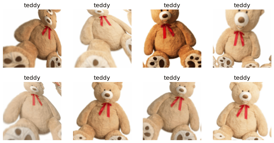
We can do this as such:
1bears = bears.new(item_tfms=Resize(128), batch_tfms=aug_transforms(mult=2))
2
3# create new `DataLoaders` object
4dls = bears.dataloaders(image_download_path)
Thus, we’ll end up with more data than the 100 images we downloaded.
6.0: Training the model
Let’s create a new DataLoaders again with our image variants.
1bears = bears.new(
2    item_tfms = RandomResizedCrop(224, min_scale=0.5),
3    batch_tfms=aug_transforms()
4)
5
6dls = bears.dataloaders(image_download_path)
FastAI has a vision_learner method which essentially allows us to further train a pre-trained model with our data. Below is the code that will train our model.
1learn = vision_learner(dls, resnet18, metrics=error_rate)
2learn.fine_tune(4)
And here is the output this produced:
| epoch | train_loss | valid_loss | error_rate | time |
|---|---|---|---|---|
| 0 | 2.242226 | 2.466239 | 0.659091 | 00:10 |
| 0 | 0.968432 | 0.818177 | 0.386364 | 00:09 |
| 1 | 0.692464 | 0.171133 | 0.045455 | 00:10 |
| 2 | 0.520085 | 0.116735 | 0.045455 | 00:10 |
| 3 | 0.424906 | 0.101607 | 0.045455 | 00:10 |
We can see that we got a very low error rate! And with just 100 images!
7.0: Cleaning up our data and retraining the model
FastAI comes with an ImageClassifierCleaner which lets us choose a category and partition of our dataset so that we can either remove images or move them to a different category. This utility does not delete or recategorise your images directly; it’ll essentially just make note of which images you chose to change. We’ll have to manually apply our changes.
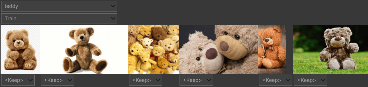
You can bring up this interface as follows:
1cleaner = ImageClassifierCleaner(learn)
2cleaner
Once you’ve gone through the images, run the following to apply your changes to the dataset:
- Remove the images you chose to delete
1for index in cleaner.delete(): cleaner.fns[index].unlink() - Move the images you re-categorised
1for index,category in cleaner.change(): shutil.move(str(cleaner.fns[index]), path/category)
Next, you’ll want to retrain your model:
1dls = bears.dataloaders(image_download_path)
2learn = vision_learner(dls, resnet18, metrics=error_rate)
3learn.fine_tune(4)
You should now hopefully see a lower error rate.
This is pretty much it with regard to training our model!
8.0: Using the model
I’ll probably go through making a more elaborate interface in the future but for now we’ll keep it simple.
If you want to use the model you just trained, you’ll have to save it. The FastAI library lets you do this with the export() method:
1learn.export()This will save the model as export.pkl. If we want to use the model, we’ll be using this file. However, before we use it, let’s download an image of a grizzly bear for us to test the model with:
1images = DDGS().images("grizzly bear", max_images=1)
2dest = 'images/grizzly.jpg'
3download_url(images[0]['image'], dest)
Now, we’ll load our model and pass it the image we just downloaded:
1path = Path()
2
3# using a model to make predictions is known as _inference_
4inference_learner = load_learner(path/'export.pkl')
5inference_learner.predict('images/grizzly.jpg')
And here’s the output the last line gave us:
('grizzly', tensor(1), tensor([1.3169e-02, 9.8664e-01, 1.9017e-04]))
This looks a bit cryptic, so we’ll break it down:
- 3 things have been returned
- the first thing,
'grizzly', is the category the model predicted out of the ones we trained it with - the second thing,
'tensor(1)', is the index of the predicted category - the last thing,
tensor([1.3169e-02, 9.8664e-01, 1.9017e-04]), tells us the probability of each category. We can see the largest value is at the 1st index (9.8664e-01), which means index 1, or the grizzly bear category, is the most probable category of the image we provided
To better understand points 3 and 4, we’ll familiarise ourselves with what the vocabulary of the DataLoaders means. This is just a list of all possible categories.
To view the vocabulary of our DataLoaders, we’ll do the following:
1inference_learner.dls.vocabThis returns the following array: ['black', 'grizzly', 'teddy']. We can see that the first index we saw above corresponds to “grizzly” in this array.
9.0: Reviewing what we did
What we just did here looks very complicated, so let’s review:
1# import and install packages
2! [ -e /content ] && pip install -Uqq fastbook
3import fastbook
4fastbook.setup_book()
5from fastbook import *
6from fastai.vision.widgets import *
7!pip install -Uqq ddgs
8!pip show ddgs
9from ddgs import DDGS1# function to get images from duckduckgo
2def search_images(keywords, max_images = 30): # max_images will default to 30
3 return L(DDGS().images(keywords, max_results=max_images)).itemgot('image')1# define bear types
2bear_types = ('grizzly', 'black', 'teddy')1# define path to download images to
2image_download_path = Path('bears')1# download 100 images for each category of bear
2if not image_download_path.exists():
3 image_download_path.mkdir()
4 for bear_type in bear_types:
5 download_destination = (image_download_path/bear_type)
6 download_destination.mkdir(exist_ok=True)
7 download_images(download_destination, urls=search_images(f"{bear_type} bear", max_images=100))1# remove corrupt images
2image_files = get_image_files(image_download_path)
3corrupt_images = verify_images(image_files)
4corrupt_images.map(Path.unlink)1# create datablock
2bears = DataBlock(
3 blocks = (ImageBlock, CategoryBlock),
4 get_items = get_image_files,
5 splitter = RandomSplitter(valid_pct = 0.2, seed = 42),
6 get_y = parent_label,
7 item_tfms = Resize(128)
8)1# apply data augmentations
2bears = bears.new(
3 item_tfms = RandomResizedCrop(224, min_scale=0.5),
4 batch_tfms=aug_transforms()
5)1# create dataloaders
2dls = bears.dataloaders(image_download_path)1# train model
2learn = vision_learner(dls, resnet18, metrics=error_rate)
3learn.fine_tune(4)1# clean data
2cleaner = ImageClassifierCleaner(learn)
3cleaner1# apply changes from data cleaning
2for index in cleaner.delete(): cleaner.fns[index].unlink()
3for index,category in cleaner.change(): shutil.move(str(cleaner.fns[index]), image_download_path/category)1# retrain model
2dls = bears.dataloaders(image_download_path)
3learn = vision_learner(dls, resnet18, metrics=error_rate)
4learn.fine_tune(4)That’s training finished! Now we’ll move onto using the model:
1# save the model to a file
2learn.export()1# download an image for testing
2images = DDGS().images("grizzly bear", max_images=1)
3dest = 'images/grizzly.jpg'
4download_url(images[0]['image'], dest)1path = Path()
2
3# let the model infer the category of our image
4inference_learner = load_learner(path/'export.pkl')
5inference_learner.predict('images/grizzly.jpg')10.0: Extrapolating what we learned
If you’d like to build a model that recognises something else, that’s pretty simple to do! Most of what you need to do is replace all of the ‘bear’ references with whatever you’re trying to search for in the code we wrote above. Before you do that though, you should modify the categories of your data. Say we wanted to build a model that distinguishes between desktop computers, laptops and phones; we’ll do the following in that case:
1device_types = ('desktop computer', 'laptop computer', 'mobile phone')
2image_download_path = Path('devices')
The rest is pretty much identical to what we did before.
Let’s test this model now:
1images = DDGS().images("iphone 4", max_images=1)
2dest = 'images/iphone.jpg'
3download_url(images[0]['image'], dest)o
4
5path = Path()
6inference_learner = load_learner(path/'export.pkl')
7inference_learner.predict('images/iphone.jpg')
The output is as such: ('mobile phone', tensor(2), tensor([2.6082e-02, 1.0686e-04, 9.7381e-01])). Works reasonably well!
10.1: Data considerations
Let’s quickly try training a model that’ll recognise the 3 most common car brands where I live: Toyota, Honda and Suzuki vehicles (any guesses where I live?).
1car_types = ('toyota', 'honda', 'suzuki')
2image_download_path = Path('cars')
3
4if not image_download_path.exists():
5  image_download_path.mkdir()
6  for car_type in car_types:
7    download_destination = (image_download_path/car_type)
8    download_destination.mkdir(exist_ok=True)
9    download_images(download_destination, urls=search_images(f"{car_type} car", max_images=200))
After downloading the images, we’ll train the model as usual.
The first red flag is the error rate we get after the first training:
| epoch | train_loss | valid_loss | error_rate | time |
|---|---|---|---|---|
| 0 | 1.848418 | 1.924796 | 0.526316 | 00:08 |
| 0 | 1.738966 | 1.517685 | 0.447368 | 00:09 |
| 1 | 1.597320 | 1.297774 | 0.315789 | 00:09 |
| 2 | 1.439774 | 1.219063 | 0.368421 | 00:09 |
| 3 | 1.280782 | 1.064873 | 0.342105 | 00:08 |
That’s a lot higher than before! Maybe it’ll get a bit better after we clean up the data…
| epoch | train_loss | valid_loss | error_rate | time |
|---|---|---|---|---|
| 0 | 1.780126 | 1.790101 | 0.702703 | 00:10 |
| 0 | 1.599073 | 1.489561 | 0.594595 | 00:08 |
| 1 | 1.561986 | 1.320968 | 0.540541 | 00:08 |
| 2 | 1.454573 | 1.068823 | 0.405405 | 00:09 |
| 3 | 1.323544 | 0.966137 | 0.405405 | 00:09 |
It got worse! What’s the problem here? Well, let’s try searching for Toyota cars online.
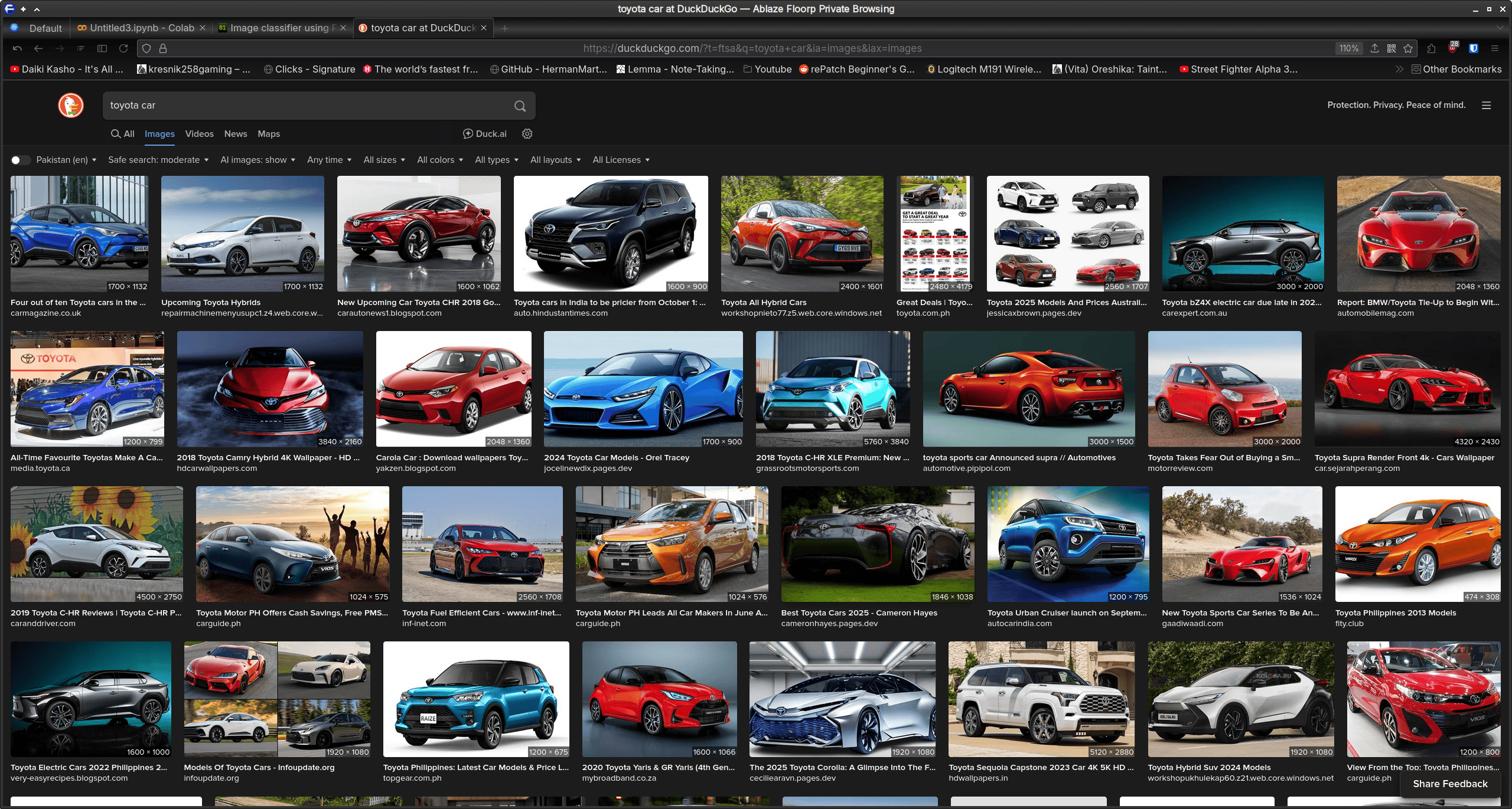
We have an almighty gaggle of images we don’t want to train our model on! For instance, traning the model on concept cars or promotional material isn’t something we want! I’d imagine this follows for the other brands too! Now, compare these results to what we get if we were to search for laptop computers as we did in our device categorisation model above:
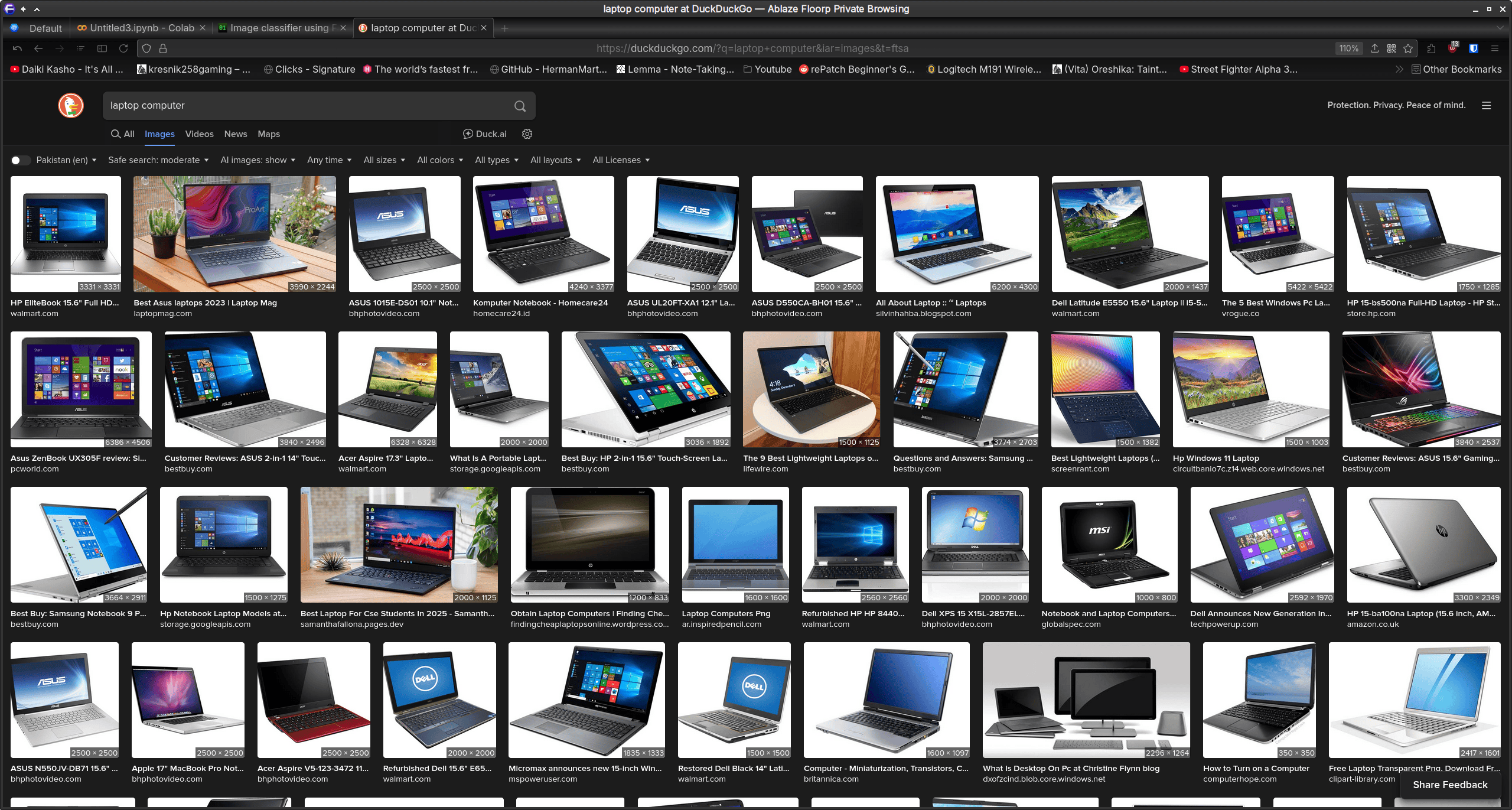
We can conclude that the data for our cars model evidently isn’t very good! But how do we know that the data is the issue here?
Well, consider that we were able to classify bears with reasonable accuracy in 4 training cycles (epochs) and from just 100 images. For these cars, we used 200 images for each while keeping the cycles the same. This should have improved! But it won’t if the data is all wonky.
Anyway, that’s that!